In recent years, we have witnessed repeated transitions from centralized to decentralized governance and vice versa. I have been involved in these changes, both in the corporate sphere in the IT field and in the field of IT solution providers. In this article, I would like to take a closer look at the transition from decentralized Data Management to centralized using Microsoft Fabric solutions. Snowflake and Apache Spark Databricks are also moving in a similar direction.
Centralized Data Management
Centralized data involves gathering data from different sources and storing it in one central database, warehouse, and data lake. The data repository offers a centralized point for managing, storing, and using data, allowing for easier maintenance and management of data.
Decentralized Data Management
Decentralized Data involves the storage, cleaning, and use of data in a decentralized way. That is, there is no central repository. Data is distributed across different nodes, giving teams more direct access to data without the need for third parties.
Comparison of Centralized versus Decentralized Data Management
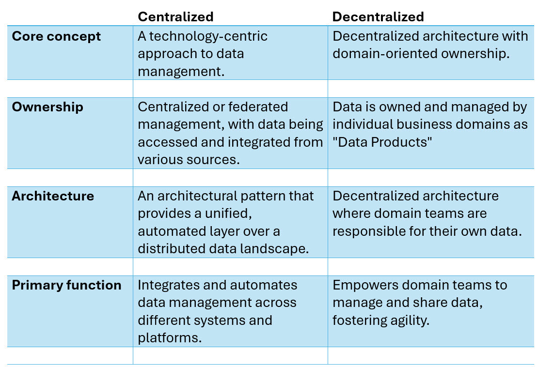
Data Mesh
is a decentralized approach to data architecture that promotes domain-oriented ownership and management of data. It advocates for treating data as a product, with each domain (or business unit) responsible for its own data pipelines, governance, and quality. The primary goal of data mesh is to address the limitations of traditional centralized data architectures by enabling scalability, agility, and autonomy of independent domains.
Data Fabric
is centralized aproach to data architecture and management. It is an end-to-end, unified analytics platform that brings together all the data and analytics tools that organizations need.
Pros and Cons of Data Fabric

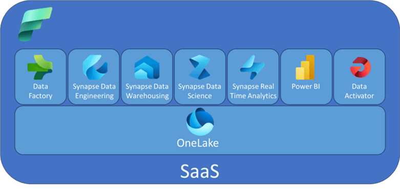
Microsoft Fabric
Microsoft Fabric is Azure's solution for a centralized Data Fabric approach It’s designed to address the challenges of a fragmented data and AI technology market by integrating various technologies like Azure Data Factory, Azure Synapse Analytics, Power BI, and OpenAI Service into a single unified product. This is a all in one analytic solution that is now covering everything from data movement to data science, real time analytics and business intelligence. And this includes everything from data lake, data engineering, data integration, Power BI, Real time analytics, and all of this is integrated in one environment. Everything is managed for us and we basically just use the software as it is (SaaS). We don't need to move the data between different tools, different services and different vendors.
Microsoft Fabric Fundamentals
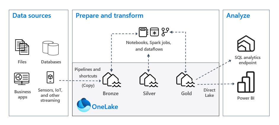
OneLake
OneLake in Microsoft Fabric serves as the central data repository, functioning like a managed data lake. Here are the key aspects of OneLake:
- Unified Storage: OneLake acts as a single, unified storage system for all your data assets. It simplifies data management by consolidating storage in one place, eliminating the need to piece together various tools and services.
- Data Accessibility: Rather than physically moving data from other locations (like AWS or Azure), OneLake allows you to create shortcuts to external files. This means you can access data without complex data pipelines, making your data management process more efficient.
- Integration: OneLake integrates seamlessly with other components in Microsoft Fabric, enabling various analytical processes without the typical barriers that exist in traditional tooling setups.
- Data Governance and Security: It includes features for data governance and security, ensuring your sensitive information is protected while providing access to authorized users within your organization.
In summary, OneLake is a highly managed data lake as a service that allows users to store, access, and manage their data effectively within Microsoft Fabric.
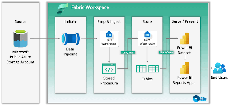
Workspace
A workspace in Microsoft Fabric acts as a dedicated environment for managing and organizing data projects. Here are the key points about workspaces:
- Segmentation: Think of a workspace as a folder or segment specifically designated for a certain project or department. This helps in organizing different types of workloads, such as data pipelines, reports, and analytics.
- Collaboration: Within a workspace, team members can collaborate on various items. The creator of a workspace typically controls who has access to it by adding users and assigning them specific roles (e.g., admin, member, contributor, or viewer).
- Creation of Items: In a workspace, you can create various data artifacts including but not limited to datasets, reports, data pipelines, notebooks, and dashboards. This allows for a comprehensive approach to data management and analysis.
- Capacity Assignment: Workspaces must be assigned to a specific capacity in Microsoft Fabric to utilize its features effectively. This capacity allows for the necessary computational power to handle the data operations within that workspace.
Overall, a workspace serves as a central hub for conducting data-related activities in Microsoft Fabric, tailored to specific needs and collaborations.
Lakehouse
A Lakehouse in Microsoft Fabric is an item created within a workspace that combines the functionalities of both data lakes and data warehouses. Here’s what you need to know about Lakehouses:
- Hybrid Storage: A Lakehouse allows you to store various types of data, including structured data (like tables) and unstructured or semi-structured data (like CSV or JSON files). This flexibility makes it suitable for complex analytics workloads and machine learning projects.
- Delta Tables: Within a Lakehouse, you can create Delta Tables, which are optimized for high performance and support both batch and real-time data processing. This enhances analytics and reporting capabilities. 3.** Centralized Location**: The Lakehouse serves as a central location for storing, managing, and analyzing files and data. This integration makes it easier to connect with other tools and processes within Microsoft Fabric.
- Compatibility and Integration: The Lakehouse integrates seamlessly with various tools and technologies, including open-source technologies like Apache Spark and Delta Lake, facilitating advanced analytics and AI-driven insights.
Overall, Lakehouses are designed to provide a flexible yet powerful data storage and management solution, bridging the gap between traditional data warehouses and modern data lakes.
SQL Analytics Endpoint
The SQL Analytics Endpoint in Microsoft Fabric is a connection interface that allows users to interact with their data stored in the Lakehouse using SQL queries*. Here are the key points regarding the SQL Analytics Endpoint:
- Connection String: The SQL Analytics Endpoint provides a connection string which can be utilized to connect other tools, such as SQL Server Management Studio (SSMS) or Power BI, to the Lakehouse. This connection string facilitates accessing tables and executing SQL queries.
- Data Preview: Through the SQL Analytics Endpoint, users can explore the data structure within the Lakehouse. You can expand schemas and view tables (e.g., a sales table) directly, allowing you to preview data visually.
- Visual Interface: The endpoint offers a visual explorer, making it easier to navigate through your data without needing to write extensive queries initially. This interface helps users to become familiar with the structure of their datasets.
- Usage in BI Tools: The SQL connection can be utilized with BI tools like Power BI, enabling users to create reports and dashboards based on the data stored in the Lakehouse.
- Integration: The SQL Analytics Endpoint is part of the unified analytics architecture in Microsoft Fabric, ensuring that data is easily accessible and manageable within a single platform.
In summary, the SQL Analytics Endpoint simplifies data interaction by providing a straightforward way for users to connect to their data and perform analytics using SQL language, enhancing the overall data management experience in Microsoft Fabric.
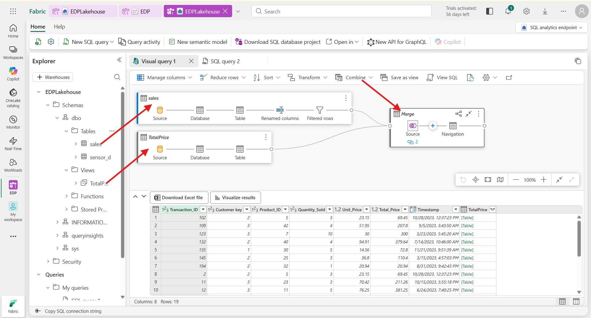
Visual Query
A visual query in Microsoft Fabric is a user-friendly tool that allows users, particularly those with less experience in SQL, to construct SQL queries using a graphical interface instead of writing code directly. Here are the key features and functionality:
- Graphical Interface: Visual queries enable users to create and manipulate queries through a visual environment. This makes it easier to understand the relationships between different data elements and to build queries without extensive SQL knowledge.
- Ease of Use: The visual query tool is designed for ease, allowing users to drag and drop elements, select tables, and specify filters or joins without needing to understand complex SQL syntax.
- Accessing Visual Query Tool: To create a new visual query, users can click on a specific icon in the interface, which opens the visual query creation options. This makes it accessible for users who might not feel comfortable with traditional coding.
- Support for Beginners: Visual queries are particularly beneficial for individuals new to data analytics or SQL, allowing them to engage with data analysis without the technical overhead of writing SQL code.
In summary, the visual query feature in Microsoft Fabric bridges the gap for users who are less familiar with SQL, providing a way to construct queries visually and efficiently.
Shortcuts
A shortcut in the context of Microsoft Fabric refers to a reference to a data table that allows you to access it without creating a redundant copy of the data. Here’s how it works:
- Definition: A shortcut acts as a link to a data table, enabling you to interact with it just like a normal table while avoiding duplication.
- Creation:
- You can create a shortcut by selecting the table you want to reference and checking the appropriate option for creating a shortcut in your workspace.
- This process allows you to connect to data from various sources, like SQL databases, and use it in a lakehouse without ingesting (copying) the data.
- Benefits: Using shortcuts prevents unnecessary data storage and allows for seamless updates; any modifications made to the original table will be reflected when accessing it through the shortcut.
- Use Cases: Shortcuts are especially useful when you want to visualize or analyze data without the need for multiple copies, ensuring that your work remains efficient and organized.
Power BI Semantic Model
The Power BI semantic model is essentially a data structure that organizes data and defines relationships between various tables, serving as a foundation for creating reports and visualizations in Power BI. Here’s a breakdown of its key aspects:
Definition: Previously known as datasets, semantic models are created when you establish a lakehouse. They centralize data management, allowing seamless access and reporting. Relationships: The semantic model maintains the relationships between different tables, which helps ensure data integrity and enables accurate data analysis in reports. Usage: You can leverage the semantic model to create Power BI reports. When setting up a report, you can select an existing semantic model as the data source, allowing you to utilize the relationships and structures defined within it. Measures: The semantic model can also include measures, which are theoretical calculations used within reports. These calculations aren’t stored physically but are computed on-the-fly when the report is run. Performance and Efficiency: By using a semantic model, you avoid data redundancy since reports directly reference the centralized data in the lakehouse. This means there’s no unnecessary duplication of data, and performance can be optimized through well-structured queries.
Overall, a semantic model enhances the ability to create effective and insightful reports within Power BI, making data analysis more efficient and coherent.
Semantic Model vs Tabular Model
The Power BI semantic model and the tabular model are both crucial elements for data analysis but serve different purposes. Here’s a breakdown of their differences and similarities:
- Definition:
- Power BI Semantic Model: This is a specific model used within Power BI that organizes and connects data from a lakehouse or other sources, allowing users to create reports seamlessly. It includes relationships between tables and serves as the foundation for visualizations.
- Tabular Model: This is generally used in SQL Server Analysis Services (SSAS) and serves as a dataset that can also operate within a multi-dimensional context. It focuses on in-memory caching for efficient querying and includes structured data in the form of tables and relationships.
- Data Storage:
- Semantic Model: Data is referenced from a lakehouse, avoiding redundancy and maintaining efficient storage. Reports leverage the centralized dataset directly without duplicating data.
- Tabular Model: Data can be stored in-memory or queried directly from a relational database. It can involve data import that might create duplicates unless effectively managed.
- Usage Context:
- Semantic Model: It is preferred for storage efficiency and centralized data management when creating reports directly in the Power BI service. Reports directly leverage this existing model.
- Tabular Model: It is often used in more advanced modeling scenarios requiring robust transformations before publishing, usually managed within a local environment like Power BI Desktop.
- Performance:
- Semantic Model: Performance can depend on whether direct query or import mode is used. It’s structured to optimize data access efficiently.
- Tabular Model: It generally provides fast query performance through in-memory data caching, but it may require additional management to optimize performance for reporting.
- Relationships:
- Both models maintain relationships between tables, essential for accurate reporting, but the management methodologies can differ. Power BI's semantic model can automatically infer relationships, making it easier to create actionable insights. In conclusion, while both models allow structured data interaction, the Power BI semantic model focuses on integration and efficiency within the Power BI ecosystem, while the tabular model is broader, used primarily in various analytical contexts.
Row Level Security (RLS)
Row-level security in Power BI is a feature that allows you to restrict data access for specific users or groups. This means different users can see different data in the same report based on their roles or permissions. Here’s how it works:
Roles Creation: You define roles within your Power BI model. Each role specifies a filter that determines what data is visible to people assigned to that role. For instance, a manager might see all data, while an employee might only see their own department's data. DAX Filters: You can use Data Analysis Expressions (DAX) to specify access rules. This involves writing DAX expressions that evaluate the current user and filter the data accordingly. User Assignment: After defining roles, you assign users to these roles either in Power BI Desktop for testing or in the Power BI service when publishing the report. Dynamic Filtering: RLS can also use dynamic filtering based on the user’s identity. This means you can automatically filter the data shown to the user based on their login credentials, which can be obtained through functions like USERNAME(), USERPRINCIPALNAME(), or ISINSCOPE().
Implementing RLS helps protect sensitive data and ensures that users see only the information relevant to them, enhancing data privacy and compliance.
Warehouse
A warehouse, in the context of data analytics, refers to a specialized layer designed for high-performance analytics and reporting on structured data. It is primarily optimized for structured data, such as relational data sourced from databases, and utilizes SQL for querying and analysis.
To break it down further:
- Purpose: Data warehouses provide strategic insights by consolidating and managing data from multiple sources, making them essential for business intelligence and reporting purposes.
- Data Structure: They are designed to handle structured data, which is organized in a format that is easily accessible and analyzable. 3.Integration with OneLake and Lakehouse: In Microsoft Fabric, data warehouses function within a broader framework that includes OneLake (a unified storage system) and Lakehouse (which combines the features of data lakes and data warehouses). This means that data warehouses can access data stored in OneLake and are suitable for performing complex analytics workloads.
- Performance: They are optimized for high-performance needs, meaning they can handle large volumes of data efficiently, making them suitable for businesses that require timely and accurate data analysis.
In summary, a warehouse is integral for organizations that need to perform robust analytics and reporting on structured data, enabling informed decision-making based on comprehensive data insights.
Diference between Lakehouse and Warehouse
The main differences between a lakehouse and a warehouse can be summarized as follows:
Data Types Supported:
- Lakehouse: Supports structured, semi-structured, and unstructured data, making it ideal for diverse data types. It allows the storage of files such as CSV or JSON alongside structured tables, providing flexibility in data management.
- Warehouse: Primarily designed for structured data, such as relational data from databases. It is optimized specifically for high-performance analytics and reporting tasks.
Architecture and Flexibility:
- Lakehouse: Combines the advantages of data lakes and warehouses, allowing for both rigid structured tables and flexible file storage. It supports real-time and batch processing for complex analytics workloads, machine learning, and data science projects.
- Warehouse: A specialized layer focused on high-performance analytics tailored for structured queries, making it familiar for traditional data analysts.
Query Capabilities:
- Lakehouse: Can be queried through a SQL endpoint, but it is read-only when using SQL, meaning you cannot perform write or update operations via SQL queries.
- Warehouse: Allows for both read and write operations, making it suitable for executing complex queries and data updates.
Use Cases:
- Lakehouse: Best suited for projects involving machine learning, real-time analytics, and processing diverse data formats. It serves as a centralized location for managing and analyzing various data types.
- Warehouse: Ideal for organizations focusing on high-performance reporting and analytics tasks that rely heavily on structured data.
In summary, the lakehouse offers a more flexible and comprehensive approach to data management, while the warehouse is specialized for efficient and performant analytics solely on structured data.

Underlying format
The underlying format of a warehouse, particularly in the context of Microsoft Fabric, involves the use of the Delta Parquet format for data storage. Here are the key points related to its underlying format:
- Delta Tables: Warehouses utilize delta tables, which are built on the Parquet format. This allows for efficient data processing and storage. Delta tables provide features like ACID transactions, efficient data updates, and schema enforcement, enhancing the reliability of data operations.
- Integration with OneLake: The warehouse operates within the OneLake storage system, which serves as a unified storage solution. This integration enables warehouses to access and utilize data stored across different formats and sources.
- SQL Support: The data warehouse environment also facilitates the use of T-SQL (Transact-SQL) for creating and managing tables, as well as for running analytics queries. This is a critical feature that distinguishes it from other components like lakehouses, where direct table creation is not supported.
- Performance Optimization: The warehouse is specifically optimized for high-performance analytics and reporting on structured data, making it suitable for traditional BI use cases.
In summary, the warehouse is constructed around delta tables in the Parquet format and is designed to deliver high-performance query capabilities while facilitating robust data management features.
Apache Spark
Apache Spark offers several strengths that make it a powerful tool for data processing and analytics:
- Distributed Computing: Spark is designed to operate across a network of machines, allowing it to efficiently handle large datasets and complex data processing tasks. This distributed nature means computations are executed in parallel, making it much faster than processing on a single machine.
- In-Memory Processing: By caching data in memory instead of relying on disk reads, Spark significantly speeds up data processing. This enables quicker access and manipulation of data, which is vital for real-time applications.
- Resilient Distributed Datasets (RDDs): Spark's core abstraction for handling data is RDDs, which are fault-tolerant collections of data partitions distributed across the cluster. RDDs ensure that data can be recovered from errors, maintaining data integrity and processing performance.
- Flexibility with Programming Languages: Spark supports multiple programming languages, including Scala, Python, and Java. This flexibility allows data engineers and data scientists to choose a language they are comfortable with, facilitating easier development.
- Support for Both Batch and Real-Time Processing: Spark can handle both batch processing and streaming data, making it versatile for different types of analytics tasks.
- Integration with Machine Learning: Spark includes libraries for machine learning, data science, and graph processing, enabling advanced analytics directly within the framework.
- Optimized for Large-Scale Data Operations: It is well-suited for processing large amounts of data efficiently, making it an ideal choice for large-scale ETL processes and analytics.
These strengths position Apache Spark as a vital tool in the toolkit of data scientists and engineers, especially when working with large and complex data environments.

Loading data from a lakehouse
To load data from a lakehouse into a DataFrame using Databricks, you can follow these steps:
- Set Up Your Environment: Make sure you have access to the lakehouse in Databricks.

- Load Data: Use Spark's read functionality to load data into a DataFrame. The syntax generally looks like this:
# Inferring the Schema Automatically

df = spark.read.format("csv") \
    .option("header", "true") \
    .option("inferSchema", "true") \
    .load("lakehouse_path")
Replace lakehouse_path with the actual path to your file in the lakehouse.
Adjust Options as Needed: Depending on your data format (e.g., CSV, JSON, Parquet), you might need to adjust the
.formatand include other options, such as delimiters or schema definitions.Work with Your DataFrame: After loading the data, you can perform various operations such as showing some rows, processing, or analyzing data:
df.show()
- Error Handling (Optional): If there’s an error loading the DataFrame, review the path and format options to ensure everything is correctly specified.
Writing a DataFrame back to a lakehouse
Prepare Your DataFrame: Ensure you have the DataFrame ready that you want to write to the lakehouse.
Write as a Delta Table: The preferred method for storing data in a lakehouse is as a Delta table. This allows for optimized performance and compatibility with tools like Power BI. You can use the following code snippet:
df.write.format("delta").saveAsTable("tablename")
Replace tablename with the name you want to assign to your table in the lakehouse.
- Write as a CSV File (Alternative Option): If you prefer to write the DataFrame as a file, such as a CSV, you can use:
df.write.csv("lakehouse_path")
Here, replace lakehouse_path with the path where you want to save the CSV file. Databricks will create the necessary directories if they do not exist.
Check the Path: For the CSV option, ensure that the path you specify is correct, as that is where the output file will be generated.
Verify the Write Operation: After the write operation, you can verify that the data has been saved correctly by reading it back into a DataFrame using:
new_df = spark.read.format("delta").load("lakehouse_path")
Temporary views
To create and use temporary views in a Databricks notebook, follow these steps:
- Create Temporary Views: You can create a temporary view using the createOrReplaceTempView method. For example, if you have a DataFrame called sales, you can create a temporary view like this:
sales.createOrReplaceTempView("sales_temp_view")
- Query the Temporary View: After creating the temporary view, you can run SQL queries against it. For instance:
result = spark.sql("SELECT * FROM sales_temp_view")
result.show()
Session Scope: Keep in mind that temporary views are session-scoped; they will only exist during the active notebook session. Once the session ends, the view will no longer be accessible.
Use Multiple Views: You can create multiple temporary views from different DataFrames. For example, if you have another DataFrame called products, you can create a temporary view for it as well:
products.createOrReplaceTempView("products_temp_view")
- Combine Queries: Temporary views allow you to run complex SQL queries involving multiple views and DataFrames, combining the power of Spark with SQL syntax for more flexibility. This approach enables effective data manipulation and querying without the need for permanent storage, facilitating quick data analysis within your current session.