Power BI DAX Masterclass

Calculated column vs Mesure

In Power BI, measures and calculated columns serve distinct purposes:

Calculated Columns:

• A calculated column creates a new physical column in your data table.
• It calculates values row by row based on a formula. Hence, it physically exists in your table.
• Use calculated columns when you need persistent data that doesn’t depend on report context. For example, these can be useful for data transformations or manipulations.

Measures:

• A measure, on the other hand, does not physically exist in the table. It is calculated dynamically when needed, typically when you visualize data in reports.
• Measures are evaluated in the context of the filters and slicers applied in your reports, allowing for more flexible and complex calculations.
• They are highly reusable across different visuals and reports, which makes them beneficial for calculations such as totals, averages, and variances.

Key Differences:

• Calculated columns operate at the row level and are static until refreshed, while measures are dynamic and depend on the visual filtering context.
• The performance can be affected by calculated columns especially when they involve complex calculations and cover large datasets.

Choosing between them depends on your specific needs for data analysis and visualization. Generally, measures are preferred for their flexibility and dynamic nature.

Date Tables

In Power BI, both the CALENDARAUTO and CALENDAR functions are used to create date tables, but they differ in their approach and flexibility:

CALENDARAUTO:

• Automatically generates a date table based on the existing date values in your model.
• It finds the earliest and latest dates in your data to create a contiguous range of dates without any missing dates.
• You don’t need to specify start or end dates, making it quicker to implement. However, it does not allow for customization of the start date or fiscal year considerations.

CALENDAR:

• Requires you to manually specify the start and end dates for the date table.
• This provides more flexibility as you can set exact dates and adjust for fiscal years.
• For example, you might call it with CALENDAR(DATE(2020, 1, 1), DATE(2025, 12, 31)) to define the exact range you desire.

Key Considerations:

• If you want an automatic date range based on your existing data without manual input, use CALENDARAUTO.
• If you need precise control over the date range and fiscal settings, opt for CALENDAR.

Date Table Script

• In our case script is based on existing table sales and column date

DateTable = 
ADDCOLUMNS ( 
CALENDAR(MINX('sales','sales'[date]),MAXX('sales','sales'[date])),
"DateAsInteger", FORMAT ( [date], "YYYYMMDD" ),
 "Year", YEAR ( [date] ), "MonthNo", FORMAT ( [date], "MM" ), 
"YearMonthNo", FORMAT ( [date], "YYYY/MM" ), 
"YearMonth", FORMAT ( [date], "YYYY/mmm" ), 
"MonthShort", FORMAT ( [date], "mmm" ),
"MonthLong", FORMAT ( [date], "mmmm" ), 
"WeekNo", WEEKDAY ( [date] ), 
"WeekDay", FORMAT ( [date], "dddd" ), 
"WeekDayShort", FORMAT ( [date], "ddd" ), 
"Quarter", "Q" & FORMAT ( [date], "Q" ), 
"YearQuarter", FORMAT ( [date], "YYYY" ) & "/Q" & FORMAT ( [date], "Q" ))

Key Measures table

Purpose:

A Key Measures table consolidates all your measures in one place, making them easier to manage and reference across your reports. This organization helps improve readability and access to all key calculations.

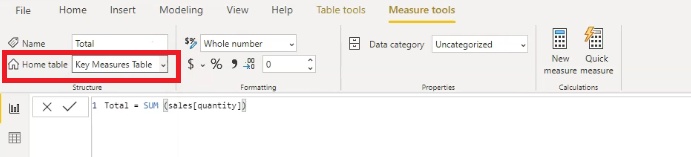
Creating the Table:

• Go to the home ribbon in Power BI.
• Click on "Enter Data" to create a new table.
• You don’t need to input any data; simply name the table “Key Measures Table”.
• Click "Load" to create the empty table.

Moving Measures:

• Once your Key Measures table is created, you can start moving existing measures into this new table for better organization.
• Select the measure you wish to relocate and change its destination to the Key Measures table.

Benefits:

By organizing your measures into a Key Measures table, you can not only make your data model cleaner but also leverage the full benefits of measure reusability across different visuals and reports. This organization aids in quicker access and clearer insights during your analysis.

COUNT Agregation functions

In Power BI, the DAX functions COUNT, COUNTA, COUNTBLANK, DISTINCTCOUNT, and COUNTROWS are important for tallying data based on different criteria:

COUNT:

Counts the number of rows that contain numeric data in a specified column. Use it when you specifically want to count only the rows that contain numbers.

COUNTA:

Counts the number of rows that are not empty in a specified column, regardless of the data type (numeric or text). Use this function when you want to count all non-blank entries.

COUNTBLANK:

Counts the number of blank rows in a specified column. This is useful to determine how many entries are missing data.

DISTINCTCOUNT:

Counts the number of unique values in a specified column, excluding duplicates. Use it when you want to analyze how many distinct entries exist in that column.

COUNTROWS:

Counts the number of rows in a table or a table expression. This function is helpful when you want to know the total number of rows available in a specific data table.

Summary:

• Use COUNT for numeric-only count.
• Use COUNTA for overall non-empty count.
• Use COUNTBLANK for counting missing data.
• Use DISTINCTCOUNT for counting unique values.
• Use COUNTROWS for total row count in a table.

X functions

In Power BI, the X functions (often referred to as iterator functions) are a powerful category of DAX functions that allow you to perform operations on rows of a table, returning a result based on each individual row's context. Here are a few key examples:

SUMX:

Iterates through a table, evaluating an expression for each row and returning the sum of those values. Use it when you want to create a cumulative total based on a calculated or derived column.

AVERAGEX:

Similar to SUMX, but instead, it computes the average of the values returned by the expression for each row in the table.

MINX and MAXX:

These functions return the smallest or largest value, respectively, from a set of values returned by an expression evaluated for each row.

###COUNTX: Counts the number of rows that contain non-blank results from the expression evaluated for each row in the table.

MEDIANX:

Returns the median of a set of values specified by evaluating an expression for each row in the table.

General Use Cases:

The X functions are especially useful for calculations that depend on row context, enabling you to iterate through tables and apply complex logic that standard aggregation functions (like SUM or AVERAGE) cannot handle by themselves.

Key Advantages:

By using iterator functions, you can create more dynamic and context-aware calculations, which can lead to deeper insights in your Power BI reports.

Using X functions can greatly enhance your DAX formulas, providing versatility and power in your data analysis. Understanding how to effectively apply these functions will significantly improve your capability to create sophisticated reports and dashboards in Power BI.

Power BI vs Excel

Power BI and Excel are both powerful tools for data analysis, but they serve different purposes and have distinct functionalities.

Data Structure:

• In Excel, calculations are centered around individual cells. You reference these cells directly to perform calculations. For instance, if you want to calculate revenue, you multiply values from specific cells.
• In contrast, Power BI operates on a model where the focus is on tables and columns rather than individual cells. The data is structured in tables with relationships between them, allowing for more complex data analysis.

Analysis Capabilities:

• Excel is great for quick calculations and straightforward data manipulation, making it ideal for smaller datasets or less complex analyses.
• Power BI excels in handling larger datasets and provides advanced analytical capabilities. It employs DAX (Data Analysis Expressions) for creating measures and calculated columns, enabling users to perform sophisticated data modeling and insights generation.

Visualization:

• While Excel offers chart and graph capabilities, Power BI provides richer visualizations with dynamic features. It allows users to create intricate dashboards that can interact with the data in real-time.

Collaboration and Sharing:

• Power BI offers enhanced features for collaboration and sharing reports online, making it better suited for team environments and organizational use.

Overall, if you need detailed visualizations and work with large datasets, Power BI is typically the better choice. For simpler tasks or if you are already experienced in using Excel, it may suffice for your needs.

Filter vs Row context

In Power BI, understanding the difference between filter context and row context is crucial for effectively using DAX (Data Analysis Expressions).

Filter Context

1. Definition: Filter context refers to the set of filters applied to the data before performing calculations. It determines which rows of data are included in the calculation.
2. Usage: An example of using filter context is through the CALCULATE function. For instance, you might use CALCULATE to compute total sales for a specific category:

• Code: TotalSalesElectronics = CALCULATE(SUM(Sales[SalesAmount]), FILTER(Sales, Sales[ProductCategory] = "Electronics")) Here, FILTER creates a new table containing only the rows where the product category is "Electronics," thereby modifying the filter context for the SUM function.

Row Context

1. Definition: Row context exists when a calculation is performed on a per-row basis. This means that for each row in a table, certain expressions are evaluated before any aggregation occurs.
2. Usage: You often encounter row context when using functions like SUMX or AVERAGEX. For example, with SUMX, it calculates an expression for each row (like quantity times price) and then aggregates those results:

• Code: TotalRevenue = SUMX(Sales, Sales[Quantity] * Sales[Price]) In this case, the expression is calculated for each row before summing the results.

Key Differentiations

• Context Transition: When you use a function like CALCULATE, it converts a row context into a filter context, allowing you to change how filters are applied to the data.
• Memory Usage: Row context calculations might require more memory, as each computed result is stored before aggregation.

Understanding these contexts will help you to build more effective DAX measures in Power BI, ultimately enhancing your data analysis capabilities.

CALCULATE function

The CALCULATE function in DAX is a powerful tool used to change the context in which a calculation is performed in Power BI. Here’s a breakdown of how the CALCULATE function works:

Purpose

CALCULATE modifies the filter context before performing calculations, allowing for nuanced data analysis based on specified criteria.

Syntax

The basic syntax of the CALCULATE function is:

CALCULATE(<expression>, <filter1>, <filter2>, ...)

• <expression>: This is the calculation you want to evaluate (e.g., SUM, AVERAGE, etc.).
• <filter1>, <filter2>, ...: These are the filters that modify the context of the calculation.

Example

For instance, if you want to calculate total sales for a specific category, the formula would look something like this:

TotalSalesElectronics = CALCULATE(SUM(Sales[SalesAmount]), FILTER(Sales, Sales[ProductCategory] = "Electronics"))

In this example:

• SUM(Sales[SalesAmount]) is the expression that computes total sales.
• FILTER(Sales, Sales[ProductCategory] = "Electronics") modifies the filter context so that only sales data for the "Electronics" category is considered.

Key Points

• CALCULATE can be used to apply multiple filters, making it flexible for various scenarios.
• It’s essential for creating dynamic measures that can adapt to different user selections and slicers in your reports.

Importance

Understanding how to effectively use CALCULATE is crucial for building robust, context-aware measures in Power BI that can provide deeper insights into your data.

FILTER function

The FILTER function in DAX is a powerful tool for creating custom filters on tables. Could be used as FILTER part of the CALCULATE function:

Purpose

The FILTER function is primarily used to return a table that includes only the rows that meet specific criteria. It operates in a way that lets you specify the filtering conditions dynamically within your DAX formulas.

Syntax

The basic syntax of the FILTER function is:

FILTER(<table>, <filter_expression>)

• <table>: The table you want to filter.
• <filter_expression>: An expression that defines the conditions that must be met for rows to be included in the returned table.

Example

Suppose you have a Products table and want to create a new table that includes only products with a price greater than $5. You would use the FILTER function as follows:

FilteredProducts = FILTER(Products, Products[Price] > 5)

In this case, FilteredProducts will contain only those rows from the Products table where the price exceeds $5.

Key Points

• Table Function: FILTER is considered a table function because it returns a table as a result. This is distinct from scalar functions, which return a single value.
• Used in CALCULATE: Often, the FILTER function is used within the CALCULATE function to modify the evaluation context of a measure. This allows you to perform calculations based on a specific subset of data.

Considerations

• Using FILTER effectively can lead to more sophisticated data analysis, allowing for greater insights by dynamically adjusting the data subsets being analyzed.
• It’s crucial to understand how it interacts with row and filter context to leverage its full potential.

ALL function

The ALL function in DAX is used to remove filters from a specified table or column. This can be particularly useful when you want to perform calculations that require analyzing the complete dataset without any applied filters.

Purpose

The ALL function allows you to ignore any filters in your context, returning the entire table or column, and is often used in conjunction with functions like CALCULATE to create metrics that require a different evaluation context.

Syntax

The syntax for the ALL function is:

ALL(<table_name_or_column_name>)

• <table_name_or_column_name>: This specifies the table or column from which you want to remove filters.

Example

1. For instance, if you want to calculate the total sales regardless of any filters applied in your report visuals, you could write:

TotalSalesAll = CALCULATE(SUM(Sales[SalesAmount]), ALL(Sales))

In this example:

• SUM(Sales[SalesAmount]) calculates the total sales amount.
• ALL(Sales) removes any filters applied to the Sales table, ensuring that the total sales calculation considers all rows in the table.

2. if you want to calculate percentage of the revenue by state filter applied in your report visuals, you could write:

Revenue filtered by a state = Revenur Mesure / CALCULATE((Revenue Measure), ALL(location[state]))

In this example:

• Revenur Mesure revenue for each column calcilated by SUMX.
• ALL(location[state]) removes any filters applied to the state of the location table, ensuring that the total revenue calculation considers all rows in the table.

Key Points

The ALL function is beneficial for creating calculated measures that need overall insights, such as calculating percentages of total sales or comparing values against grand totals. Different variations of ALL exist, including ALLSELECTED, which removes filters but keeps the filters applied by the user’s selections in slicers or visuals. Using the ALL function allows for a more profound and comprehensive analysis across your data.

ALLSELECTED function

The ALLSELECTED function in DAX is used to remove filters from columns or tables while still considering any filters applied in the current report context, such as slicers, without disregarding selections made by the user.

Purpose

It enables you to compute values over a specified range of data, which may involve filters from the visual elements of the report but not those defined in the measure itself.

Syntax

The syntax for ALLSELECTED is:

ALLSELECTED(<table_name_or_column_name>)

• <table_name_or_column_name>: This is the specific table or column for which you want to retain the filters from the user’s selections while removing others.

Example

Suppose you want to calculate the percentage of sales compared to total sales considering only the filters from slicers. You could use:

SalesPercentage = DIVIDE(SUM(Sales[SalesAmount]), CALCULATE(SUM(Sales[SalesAmount]), ALLSELECTED(Sales)))

In this formula:

• SUM(Sales[SalesAmount]) calculates the sales for the current context.
• ALLSELECTED(Sales) removes any filters on the Sales table but respects filters from slicers, ensuring that the calculation reflects the intended scope.

Key Points

ALLSELECTED is particularly useful for creating responsive measures in reports where user interaction (like slicers or filters) needs to modify results dynamically while still allowing a full range of data to be analyzed. It provides flexibility when crafting insights that depend on user-driven contexts, such as dashboards where users might want to see insights filtered by certain criteria while still maintaining a broader view of the data.

ALLEXCEPT function

The ALLEXCEPT function in DAX is used to remove filters from all columns in a table except for the specified columns. This function is particularly useful when you want to maintain certain filters while disregarding others during calculations.

Purpose

The ALLEXCEPT function is ideal when you want to summarize data while keeping specific dimensions in the filter context, allowing for more targeted analysis.

Syntax

The syntax for ALLEXCEPT is:

ALLEXCEPT(<table>, <column_1>, <column_2>, ...)

• <table>: The table from which to remove all filters.
• <column_1>, <column_2>, ...: The columns that you want to keep the filters for.

Example

For instance, if you have a Sales table and want to calculate the total sales while keeping the filter for Region, you might write the following:

TotalSalesByRegion = CALCULATE(SUM(Sales[SalesAmount]), ALLEXCEPT(Sales, Sales[Region]))

In this example:

• SUM(Sales[SalesAmount]) computes the total sales.
• ALLEXCEPT(Sales, Sales[Region]) allows the Region filters to remain while ignoring other filters in the Sales table.

###Key Points ALLEXCEPT is useful for creating measures that need to respect specific dimensions while performing calculations over the entire dataset. It helps in scenarios where you want to create comparisons (e.g., percentage calculations) that focus on certain filter aspects without losing other important insights from your data.

Logical Operators

In DAX, logical operators allow you to create complex filtering conditions in your calculations. Here are the primary logical operators used in DAX:

1. AND Operator (&&) The AND operator is used to combine multiple conditions, where all conditions must be true for the entire expression to evaluate to true. Example:

IF(Sales[Amount] > 1000 && Sales[Region] = "North", "High Sale", "Low Sale")

2. OR Operator (||) The OR operator allows for conditions where at least one of the conditions must be true for the expression to evaluate to true. Example:

IF(Sales[Amount] < 500 || Sales[Region] = "South", "Low Sale or in South", "Regular Sale")

3. NOT Operator (NOT) The NOT operator is used to negate a condition. If the condition is true, NOT makes it false and vice versa. Example:

IF(NOT(Sales[Region] = "East"), "Not in East", "In East")

4. Combining Conditions You can combine these logical operators to create more complex conditions. However, be mindful of the order of operations; the AND operator is evaluated before the OR operator. Example:

IF((Sales[Amount] > 1000 && Sales[Region] = "North") || (Sales[Amount] < 500), "Specific Sale Condition", "Other")

Usage in Filtering

These operators are often used with functions like CALCULATE to create dynamic measures based on complex filtering criteria. For example, you could filter a dataset to include products that are either above a certain price point or within a specific category, as mentioned in the course where the operator logic was discussed.

Understanding how to effectively use logical operators can help you build sophisticated analytics in your DAX queries.

VALUES and AVERAGEX function

The VALUES function and the AVERAGEX function in DAX serve distinct purposes but can work together effectively in your calculations.

VALUES Function

The VALUES function returns a one-column table that contains the distinct values from the specified column or table. It can be used to create a unique list of values for further calculations. Example Use: If you want to get a list of unique values from a date column, you would use:

VALUES(DateTable[Date])

AVERAGEX Function

The AVERAGEX function iterates through a table, evaluating an expression and returning the average of those values. It is an iterator function, meaning it processes each row of the table specified. Syntax:

AVERAGEX(<table>, <expression>)

Example Use: To calculate the average sales amount by iterating over a table of sales data:

AVERAGEX(SalesTable, SalesTable[SalesAmount])

Combining VALUES and AVERAGEX

You can combine these two functions to calculate averages based on distinct values. For example, to calculate the monthly average revenue, you could write:

MonthlyAverageRevenue = AVERAGEX(VALUES(DateTable[YearMonth]), [RevenueMeasure])

In this case: VALUES(DateTable[YearMonth]) provides a unique list of year-month combinations, and for each combination, the [RevenueMeasure] is evaluated and averaged. This combination allows for powerful analytics where averages are calculated based on distinct segments of your data, providing insights tailored to your reporting needs.

RANKX function

The RANKX function in DAX is used to rank values within a specified context. It allows you to determine the rank of an expression evaluated for each row across a table. This is particularly useful for identifying top-performing items based on a certain measure, such as revenue.

Purpose

The RANKX function assigns a rank (1 for the highest value, 2 for the next highest, etc.) to each row in a specified table based on the evaluation of an expression.

Syntax

The syntax for RANKX is:

RANKX(<table>, <expression>, [<value>, <order>])

• <table>: The table containing the values to rank.
• <expression>: The expression to evaluate and rank.
• <value> (optional): An optional value that you can provide when the expression returns a blank.
• <order> (optional): Sort order (0 for descending, 1 for ascending; defaults to descending).

Example

For example, if you want to rank customers based on their quarterly average revenue, you might create a measure like this:

Ranking by Quarterly Average = CALCULATE( RANKX ( ALLSELECTED( customer ) , [Quarterly Average Revenue] ) ,
ALL ( DateTable[Year] ) )

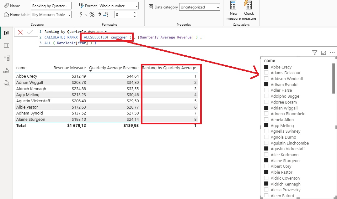
In this example:

• ALLSELECTED( customer ) is the table we are ranking with customer slicer applied.
• [QuarterlyAverageRevenue] is the measure for which ranks are calculated.
• ALL ( DateTable[Year] ) - remove all filters based on Year of the DateTable table

Practical Use

• You can use RANKX in tandem with other measures to filter the top performers or analyze performance over time. For instance, to filter and see only the top ten customers ranked by quarterly average revenue, you could create a calculated table or fit this measure in a visual filter.
• Combining RANKX with a helper table, such as a Top N filter, can also improve your analysis by giving you dynamic control over how many top-ranked items to display.

IF function & Top-N filter

The IF function in DAX can be effectively used in conjunction with a Top-N filter to dynamically filter data based on ranking. Here's how you can implement a Top-N filter using an IF statement.

Creating a Top-N Filter

1. Helper Table: First, create a helper table that specifies your Top-N options such as Top 3, Top 5, Top 10, etc. This table will allow you to control how many entries you want to see in your report.

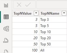
2. Creating the Measure: You will then need to create a measure that utilizes the ranking and implements the IF statement to determine whether to include a particular value based on its rank.
3. Sample Measure: Here’s an example of how you might create a measure that filters to only show revenue for the top N ranked customers:

TopN Revenue = IF ( [Ranking by Quarterly Average] <= MAX(TopNFilter[TopNValue]) , 
	[Revenue Measure] , 
	BLANK() ) 

In this example, [Ranking by Quarterly Average] is the measure that calculates the rank, and [RevenueMeasure] calculates the revenue. The IF statement checks if the rank is within the specified Top-N value.

How It Works

• The measure calculates the ranking for each customer and then checks if it falls within the defined Top-N range. If true, it returns the corresponding revenue; if false, it returns a blank.
• This allows for flexible reporting and analysis where you can easily adjust the Top-N filter to view different segments of your data.

Practical Application

Using this approach, you can dynamically analyze which customers, products, or any entities perform within the top range based on your chosen criteria, enhancing your insights into business performance.

Variables

In DAX, variables are a powerful feature that allows you to store values and expressions for later use within a formula. This enhances the readability and maintainability of your DAX code, and can also improve performance by avoiding repeated calculations.

Creating Variables

You can define variables in a DAX formula using the VAR keyword followed by an assignment, and then use these variables in the subsequent calculations. The structure is as follows:

MeasureName = 
VAR VariableName = Expression
RETURN
    AnotherExpressionUsing(VariableName)

Example

Here's a practical example of using a variable in a measure designed to calculate total sales while excluding a specific product category:

TotalSalesExcludingCategory = 
VAR TotalSales = SUM(Sales[SalesAmount])
VAR ExcludedSales = CALCULATE(SUM(Sales[SalesAmount]), Sales[Category] = "ExcludedCategory")
RETURN
    TotalSales - ExcludedSales

In this example:

• TotalSales holds the total sales amount.
• ExcludedSales calculates sales for a category that needs to be excluded.
• The measure subtracts ExcludedSales from TotalSales and returns the result.

Benefits of Using Variables

• Improved Readability: Using variables makes your DAX formulas easier to understand.
• Performance: Instead of calculating the same expression multiple times, you calculate it once and reference it through the variable.
• Complex Calculations: Helps in breaking down complex calculations into simpler parts, making debugging easier.

Time Intelligence & DATEADD

The DATEADD function in DAX is a powerful Time Intelligence function used for shifting dates by a specified number of intervals, which can be days, months, quarters, or years. This function allows you to create calculations that compare data from different time periods, making it essential for time-based analysis.

Syntax

The syntax for DATEADD is:

DATEADD(<dates>, <number>, <time_unit>)
<dates>: A column that contains dates.
<number>: The number of intervals to add (can be negative for subtraction).
<time_unit>: The interval to use (e.g., DAY, MONTH, QUARTER, YEAR).

Example

For instance, if you have a measure that calculates revenue, and you want to see the revenue from two days ago, you can use DATEADD like this:

RevenueTwoDaysAgo = 
CALCULATE(
    [RevenueMeasure],
    DATEADD(DateTable[Date], -2, DAY)
)

In this example:

• [RevenueMeasure] is the measure you're calculating. -DateTable[Date] is the date column, and -2 specifies to go back two days.

Use Case

The DATEADD function is particularly useful when you want to create reports that compare current metrics with those from previous periods. By shifting the context of your calculations, you can easily compute growth rates, year-over-year changes, and other time-based insights.